Geiger on a Plane
What
The atmosphere acts as a decent filter against the cosmic rays . The higher the
altitude, the less amount of air between the space and the sensor, the less filtering,
and therefore more radiation. Even then, the dose per flight for passengers tends to be rather
negligible
. The higher the
altitude, the less amount of air between the space and the sensor, the less filtering,
and therefore more radiation. Even then, the dose per flight for passengers tends to be rather
negligible , and only a rather
small concern for the aircraft crews. (See also here.)
, and only a rather
small concern for the aircraft crews. (See also here.)
The dose can be calculated using online tools.
(The route dose, using this tool, was calculated to be 9.1 microsievert.)
Why
Ummm... Because it's there?
A pancake-probe Geiger counter was built earlier. One day, the unit
was traveling to Ireland in a cabin luggage and was switched on at the cruising altitude
for the sake of curiosity. The clickety-click sound was so lively in comparison with sea level
it caused strong interest and correspondingly strong temptation.
was built earlier. One day, the unit
was traveling to Ireland in a cabin luggage and was switched on at the cruising altitude
for the sake of curiosity. The clickety-click sound was so lively in comparison with sea level
it caused strong interest and correspondingly strong temptation.
Results
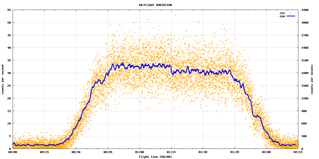
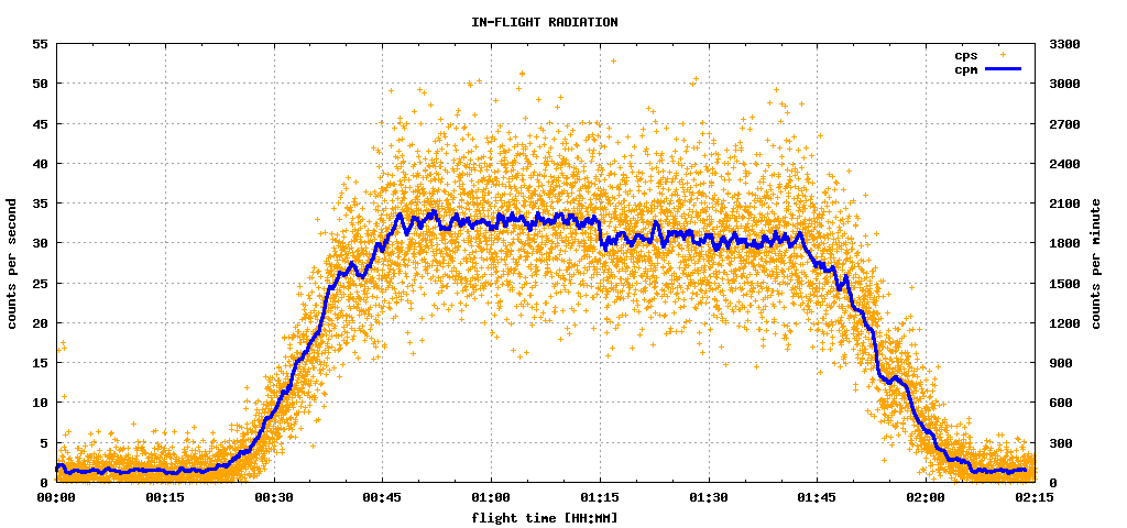
Radiation measurement of Dublin-Prague flight, 21st July 2012, approx. 11:00-13:15 (GMT+1)
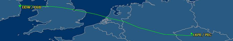
Flight altitude profile and path for Aer Lingus Teoranta (EI) #644 > 21-Jul-2012 > EIDW / DUB - LKPR / PRG
(data obtained from FlightAware, EDT timezone (GMT-4), direct link
here)
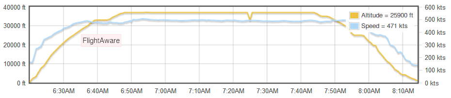
Notice the correspondence of plateaus on the ascend/descend phases of the radiation level with plateaus
on the flight altitude profile. The small but significant cpm drop since flight time 1:15 may be explained
by flying into an area with higher atmospheric pressure and correspondingly better cosmic ray absorption.
- Recorded file, MP3 (16kbps) version, 16 megabytes: geiger.mp3

- Recorded file, WAV (16ksps) version, 247 megabytes: on request
Hardware and procedure
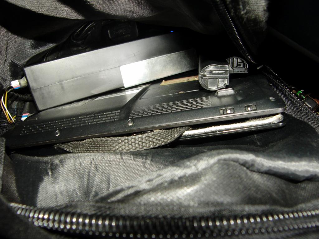
On the way back, a datalogging rig was improvised from the available hardware and software.
A netbook was wired to the Geiger, via direct connection of the counter's headphones output
to the netbook's microphone input. Audacity was used as the
software of choice for recording the sound.
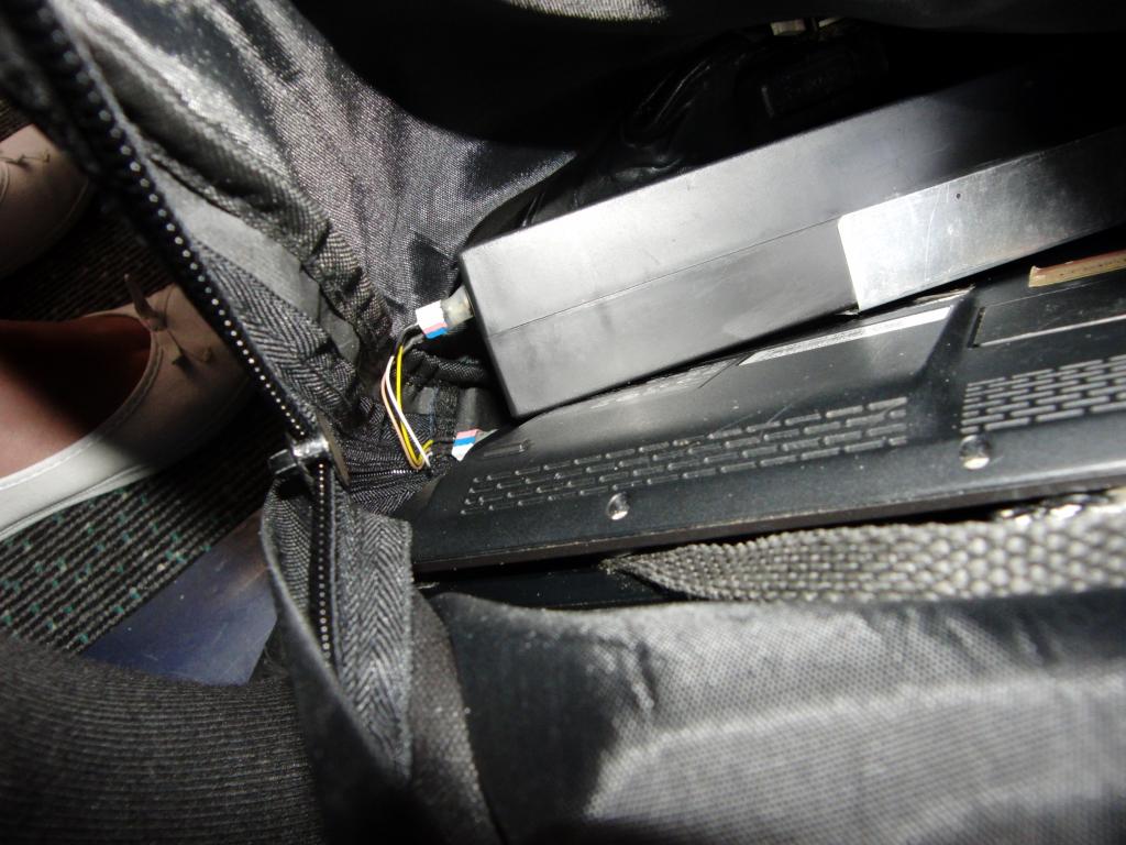
The Geiger and the netbook were connected together. Immediately after boarding the plane
the netbook was booted up, Audacity was started, and recording was set to single-channel with
16,000 Hz samplerate (this was guessed as a compromise between data file size and temporal
resolution; it turned out to be a good choice). The netbook lid was then closed (the machine's
power configuration was set to switch off the display but keep running normally) and the assembly
was concealed in the cabin luggage, where it remained for the duration of the flight.
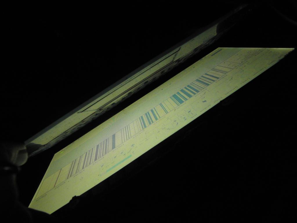
The netbook was checked a few times during the flight (partly open the lid, press a shift key
to wake the screen up, check if the recording pointer scrolls through the track window and the
waveform being recorded indicates presence of signal, close the lid).
After landing, the netbook was released from the luggage, opened, the recording was stopped,
the project was saved and the audio recording was exported as a .wav file. Then the hardware
was switched off.
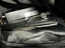
Geiger and netbook in the bag | 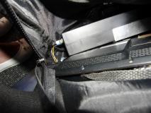
Geiger and netbook in the bag | 
In-bag netbook screen check | |
Data processing
Capture file
The acquired data file is a 16-bit .wav file, with 247 megabytes of data. The strong output of
the Geiger overloaded the input, causing clipping of the signal; this turned
out to be a major advantage during subsequent processing.
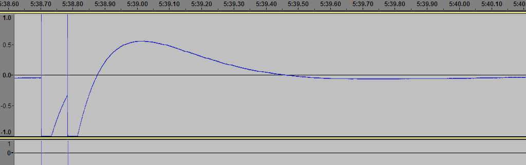
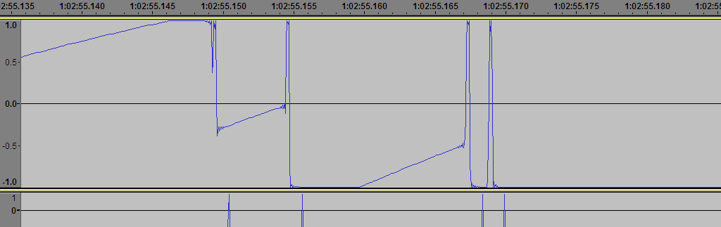
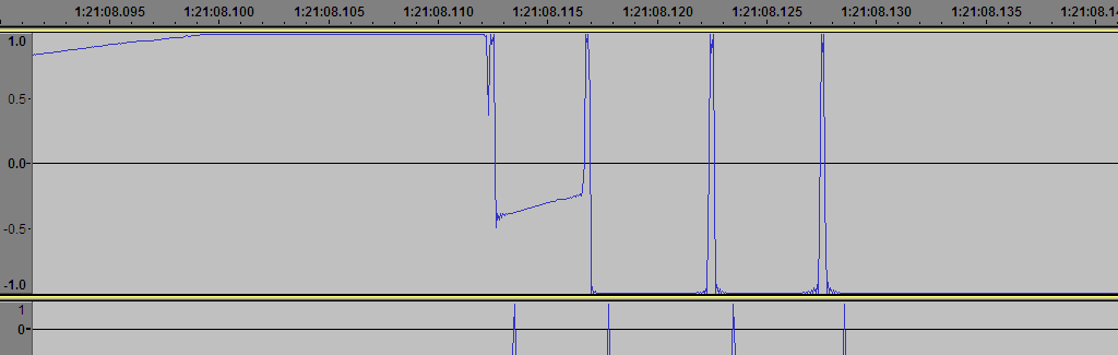
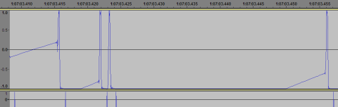
The AC coupling of the microphone input of the sound card influenced the recorded waveform; an event
is typically recorded as a rise to upper signal level limit (+1.0), immediate fall to lower limit (-1.0),
then slow return to neutral level via a smooth curve; in absence of any events for significant period,
the signal steadies itself in the middle of range (zero).
The choice of software and hardware was dictated by available resources; the idea to do the recording was
an impulse one and the experiment therefore had to be heavily jury-rigged.
Event detection
The file was converted from 16-bit .wav to a raw unsigned 8-bit format, using SoX. The resulting
file had 129,598,240 bytes. The raw 8u format is much easier for processing.
This raw file was then processed with a custom-made C program, procfile.c. (The filename is hardcoded,
output is redirected from stdout to file. Each event is marked as a 0xF7 value, otherwise the file value is 0x00.)
Both the raw 8bit file and matching event-detection file were opened in Audacity and compared side by side,
to make sure the algorithm used for event detection works as designed.
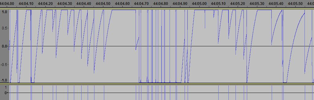
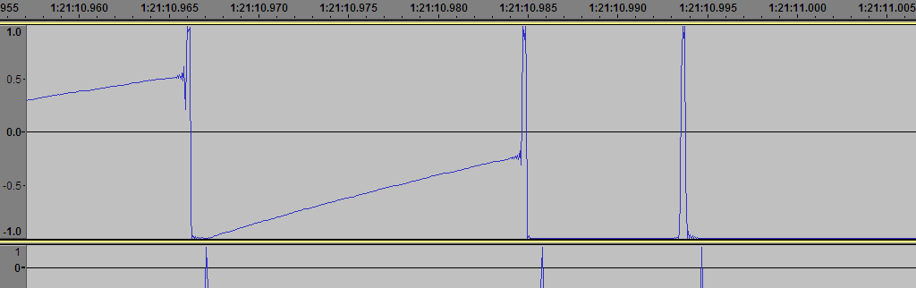
The falling edge of the signal, beginning at upper limit and staying low for at least five samples, was used as
the criterium for event presence.
Event counting
The procfile.c was used as a basis for makecount.c, which goes through the raw file and uses the same event
detection algorithm. The events are counted for each 16,000-sample interval (or, every second) and outputted
to stdout, redirected to cps.txt (counts-per-second) file.
As the cps values are scattered through a wide range, conversion to less-fluctuating value was desired.
The cps.txt file was processed by stripping the seconds-index and leaving only the raw count, cps.lst file.
A program, mksmoothcpm.c, was written to calculate a moving sum of 60 cps values for every second.
First, the cps.lst is read line by line into an array. Then, for every second, the sum of subsequent 60 array
items was calculated and outputted, resulting in a cpm-smooth.txt file with smoothly changing count-per-minute values,
calculated by second.
Screenshots
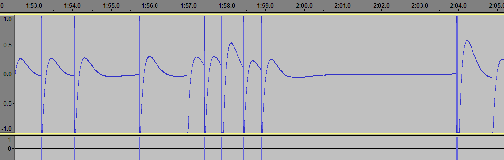
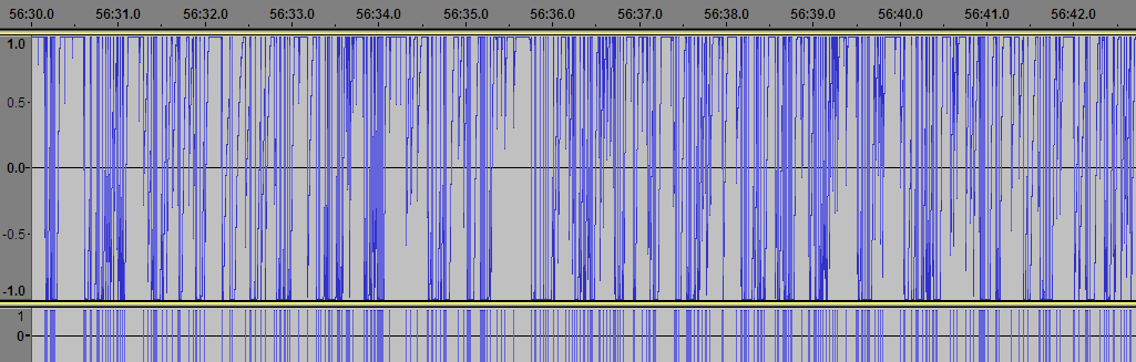
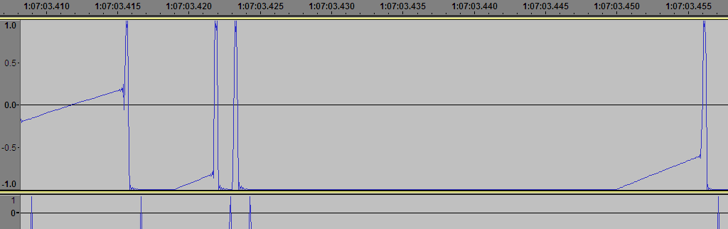
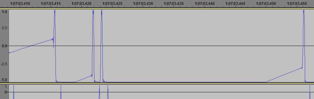
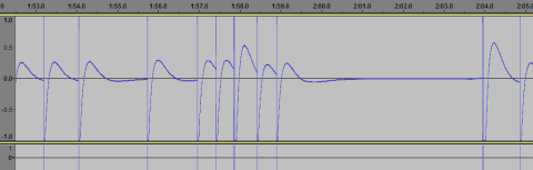
Screenshots of Audacity file view; upper trace shows the raw signal, lower trace shows the identified events.
Low-rate signal | 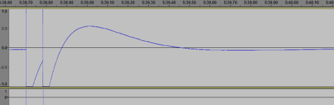
Low-rate signal, detail | | |
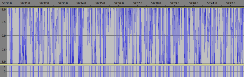
High-rate signal | 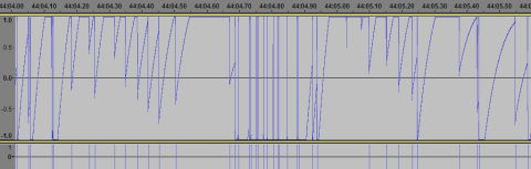
High-rate signal, detail | | |
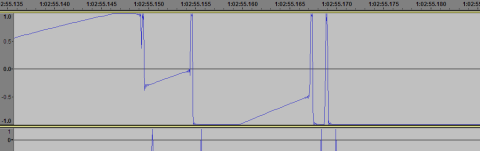
High-rate signal, ultra-detail | 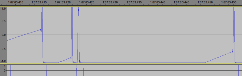
High-rate signal, ultra-detail | | |
High-rate signal, ultra-detail | 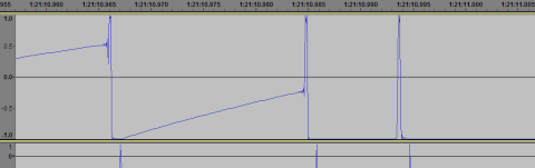
High-rate signal, ultra-detail | | |
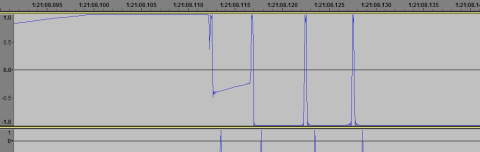
High-rate signal, ultra-detail | | | |
Graph making
For converting the measurements to a graph form, gnuplot was used. A script, makegraph.sh, was written for that
purpose, using cps.txt and cpm-smooth.txt files as data sources.
The cps values are scattered rather wildly, due to the short measurement interval and random nature of the signal. They are
displayed as orange cross marks. As the lower vertical resolution of the y2 axis together with small size of the symbols
caused the orange marks to form bands, a random noise of +-0.5 was added to the cps to avoid this visual ugliness and create
an easier-to-read point-cloud.
The smoothed cpm values are drawn as a thick blue line. The line ends a minute before the orange points do, as it is the sum
of the current second and the next 59 ones.
There are few high (15-20) cps values in the first two minutes. These are a result of artefacts brought into the recorded
signal probably by manipulations with connectors during concealment of the hardware setup.
TODO
- Build a scintillator-based gamma spectrometer. Repeat the experiment, acquire energy spectrum.
- Try with a neutron detector.
- Acquire flight path altitude profile (GPS?), correlate radiation level with altitude and latitude
- More measurements during different solar activities
Note
The source .wav file can be provided for request. Its size is too large to leave for casual downloads.
| If you have any comments or questions about the topic, please let me know here: |